Empty Shelf Detection with Keras

The Data

Here is a little info about the data. I had originally scraped google images, searching for frontal view photos of supermarket shelves. I indexed terms like ‘empty supermarket shelf’ and ‘empty Walmart shelf’, and everything similar. However, this gave us a couple of issues. Some of the data was either too artsy, or the angle was too extreme. So a lot of filtering and image augmentation had to be done. However, a couple of weeks later we got lucky and found a paper willing to share their data with anyone who asked… So we did that. You can find the paper, and the wonderful work they are doing here.

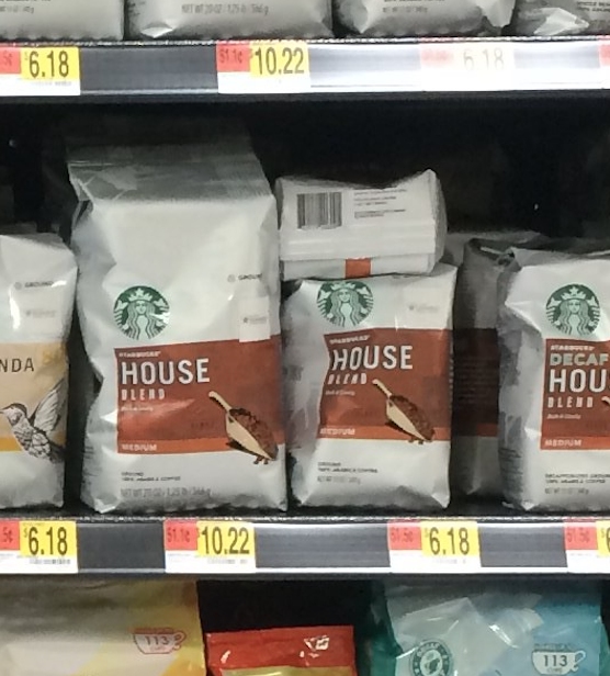
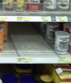
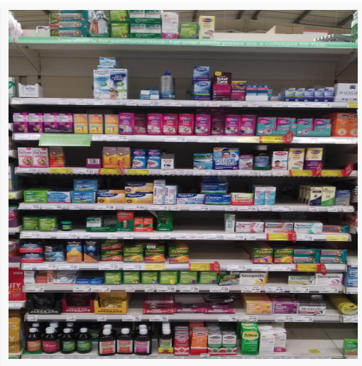
The images show some training data for the model. Because an original image can contain all three classes, I cropped sections of images to help training along. The first image shows an instance of the stocked class, the second image shows an instance of the not stocked class, and the last image shows an instance of the other class.

The Model

The model is an extension of a VGG19. That is, the first 23 layers are exactly VGG19, and the last 3 layers are trained dense layers with dropout for regularization. The last layer is 3 neurons with a softmax activation.

I initially trained on my local machine. It took about 2.5 hours to train one epoch, so I realized that I needed more processing power, and fast. Luckily, Google offers free GPUs for anyone who is willing to get their hands dirty. I got set up in Google Colab, and within 30 minutes, I was able to train 100 epochs.

base_model=VGG19(weights='imagenet',include_top=False) #imports the VGG model and discards the last 1000 neuron layer.


x = base_model.output
x = GlobalAveragePooling2D()(x)
x = Dense(512,activation='relu')(x) 
x = Dropout(0.5)(x)
x = Dense(512,activation='relu')(x) #dense layer 2
x = Dropout(0.5)(x)

preds = Dense(3,activation='softmax')(x) #final layer with softmax activation
model = Model(inputs=base_model.input,outputs=preds)

Let’s keep the model architecture pretty simple. We add dropout layers after ever dense layer, to reduce overfitting and allow us to train for more epochs. The three classes we are predicting are:

• Stocked

• Not Stocked

• Other

The first thing we need to do is freeze the VGG19 layers, and make our custom layers trainable. We can do that with the following snippet of code.

# Freeze the VGG19 Layers and keep Dense Layers trainable
for layer in model.layers[:23]:
    print(layer.name, False)
    layer.trainable=False
    
    
for layer in model.layers[23:]:
    print(layer.name, True)
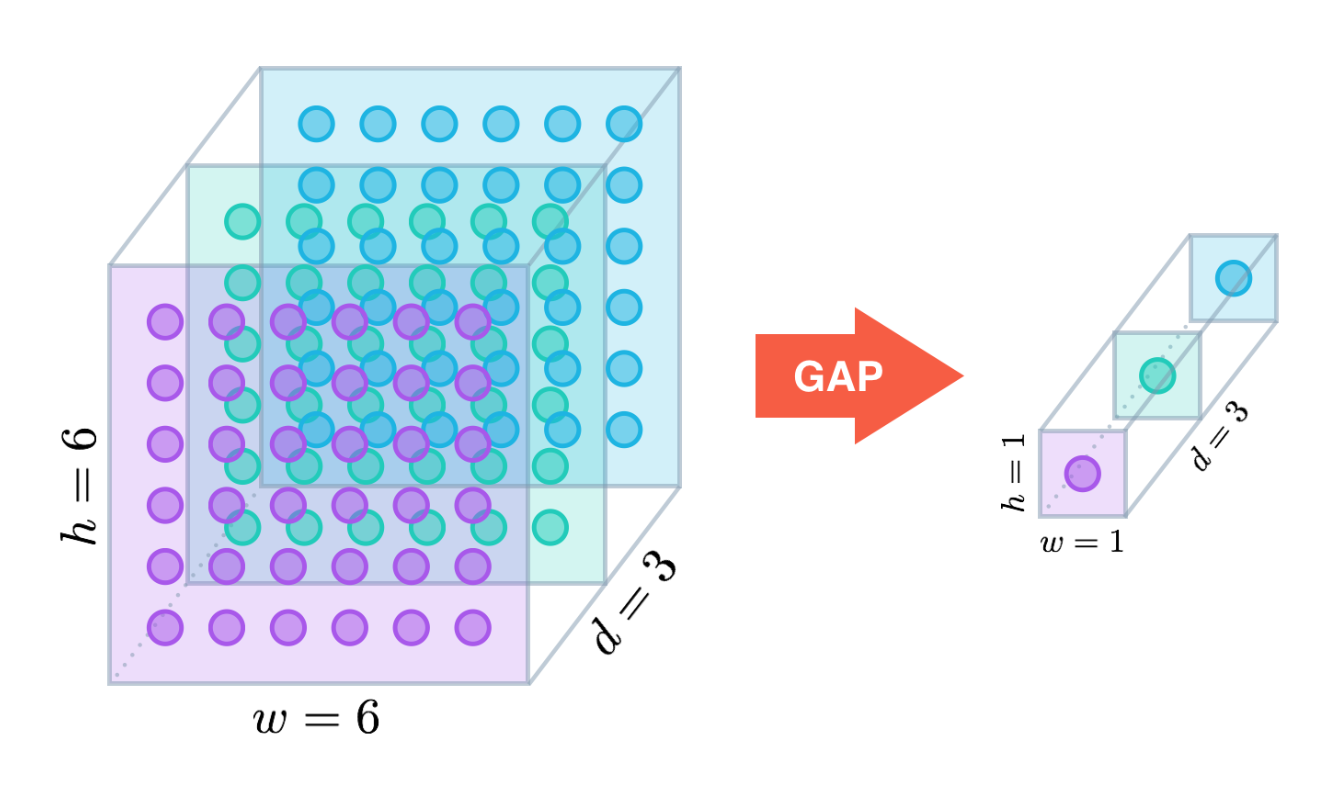
    layer.trainable=True

The first 23 layers are VGG19 + Global Average Pooling (GAP) layer. We don’t want to train these layers; in fact, we don’t want to touch these layers at all. So we set the trainable attribute to False.

The GAP layer is a way of reducing the dimensionality of the model. It essentially averages over a single color channel as so.

Now that we have the model architecture with its trainable layers, let’s start training. I’ll use a data generator to get some random augmentations thrown in there. This will help us out with overfitting as well. This will also help if we have a very large sample size, so we don’t have to store everything in memory.

train_datagen = ImageDataGenerator(preprocessing_function=preprocess_input,
                                 rotation_range=40, # Rotation +/- up to 40 degrees
                                 width_shift_range=0.3, # horizontal shifting +/- up to 30%
                                 height_shift_range=0.3, # vertical shifting +/- up to 30%
                                 zoom_range=0.3) # Magnification and shrinking +/- 30%
                                 
                                 
validation_datagen = ImageDataGenerator(preprocessing_function=preprocess_input) # For the validation data

I’m going to set up a callback function as well, so after every epoch, we save the current model. There are other ways to save the model, like having a model checkpoint based on accuracy, but let’s keep it simple for now. We will use the ModelCheckpoint module in keras. Now, all we need to do is compile the model and train.

# Callback Function
mc = keras.callbacks.ModelCheckpoint('saved_weights_path/weights{epoch:03d}.h5', 
                                     save_weights_only=True, period=1)

# Step size and train model
step_size_train=train_generator.n//train_generator.batch_size
step_size_validation = validation_generator.n // validation_generator.batch_size
mobilenet_fit = model.fit_generator(generator=train_generator,
                                    steps_per_epoch=step_size_train,
                                    epochs=100, # Change to make epochs more
                                    validation_data = validation_generator, # Also must include validation generator
                                    validation_steps = step_size_validation, # Complimenting the validation generator
                                    callbacks = [mc] # Sets the callback fucntion from before)

Localization

The method we use for localization requires a few steps:

First:

• Convert our model’s dense layers into equivalent convolutional layers. Our new fully convolutional will allow us to have any input size.
• Create some scales for the image. For each scale, perform the following:

And that’s essentially it! I’ve yadda yadda’ed over some details, but you get the picture. Heres the code.

def localizee(model,unscaled, W = 300, H = 300, THRESHOLD = .8, EPSILON = 0.02):
    """
    This function iterates through scales for a fixed w, h image and gets a heatmap. 
    The function returns a list of bounding boxes over the scales.
    It thresholds the heatmap at .8, and appends to a list.
    This function follows from: https://github.com/lars76/object-localization/blob/master/example_3/test.py
    """
    scales = np.power(0.8, np.arange(0, 5)) #[0.3, 0.4,..., 0.9, 1.0]
    list_of_heatmaps = []

    
    
    IMAGE_SIZE = 224
    
    bounding_boxes = [] #return list of bounding boxes w/ corrosponding scale
    if unscaled is None:
        #No image found
        print("No such image")
        return
    image = cv2.resize(unscaled, (IMAGE_SIZE, IMAGE_SIZE)) #(300,300)
    for i,scale in enumerate(scales[::-1]):
        #Scale the image
        image_copy = image.copy() 
        unscaled_copy = unscaled.copy()
        feat_scaled = process_pred_img(image_copy, w = int(W*scale), h= int(H*scale) )

        region = np.squeeze(model.predict(feat_scaled))
        output = np.zeros(region[:,:,0].shape, dtype=np.uint8)
        
        output[region[:,:,0] > THRESHOLD] = 1 
        output[region[:,:,0] <= THRESHOLD] = 0
            
        _,contours, _ = cv2.findContours(output, cv2.RETR_TREE, cv2.CHAIN_APPROX_SIMPLE)
        
        for cnt in contours:
            approx = cv2.approxPolyDP(cnt, EPSILON * cv2.arcLength(cnt, True), True)
            x, y, w, h = cv2.boundingRect(approx)
            try:
                #Sometimes output is a scalar and has no shape
                x0 = np.rint(x * unscaled.shape[1] / output.shape[1]).astype(int)
                x1 = np.rint((x + w) * unscaled.shape[1] / output.shape[1]).astype(int)
                y0 = np.rint(y * unscaled.shape[0] / output.shape[0]).astype(int)
                y1 = np.rint((y + h) * unscaled.shape[0] / output.shape[0]).astype(int)
            except Exception as e:
                continue
            
            bounding_boxes.append((x0, y0, x1, y1))
            cv2.rectangle(unscaled_copy, (x0, y0), (x1, y1), (255, 0, 255), 10)

    return np.array(bounding_boxes)

After this, perform Non-Maximum suppression, as described here.

When you’re done, you should have something similar to this:

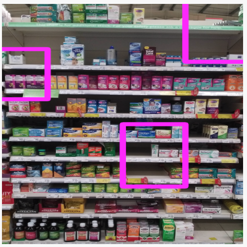
It’s not 100% perfect. In fact, it’s far from perfect, but it’s a good start, and that’s all we need for now.

Production

Assuming you have a model, we can start to productionize it. I’m going to use the Flask framework, along with a template that I found, just to because I need to brush up on my UI/UX skills, and it’s not the main purpose of this blog.

You can use git clone https://github.com/mtobeiyf/keras-flask-deploy-webapp and open up the app.py file. You should see a global model_predict function and some decorators for the routes. I will not show any code, because it’s very straightforward to use.

The main idea is to upload a user’s photo, save the photo, then call the model prediction functions that we set up. Once the predictions finish, localize, and return the new localized photo’s URL. If you want to take a peek at the code I have, look no further.