Predicting Churn with KNN
By Jamel Thomas
Although there are many examples, churn prediction is one of the classical applications of Data Science that works. Churn prediction gives businessmen and bussinesswomen the power to catch those consumers who are likely to leave the company. They can in turn take appropriate measure to keep their business. In this project, we consider a dataset of 7,043 observations. The goal here is to predict, with a fair amount of accuracy, which observations are likely to churn.
Exploratory Data Analysis
## Loading required package: ggplot2## Loading required package: magrittrNote that the echo = FALSE parameter was added to the code chunk to prevent printing of the R code that generated the plot.
DT::datatable(churn[,c(1:2,16:21)])Including Plots
You can also embed plots, for example:
my.data <- cbind(churn,data.frame(num = 1) )
my.data$SeniorCitizen <- factor(my.data$SeniorCitizen)
my.data2 <- aggregate(num~. , data = my.data[, c(7:8, 12, 16,21, 22)], sum)


SankeyDiagram(my.data2[, - dim(my.data2)[2]],
              link.color = "Source",
              weights = my.data2$num)
temp <- churn[churn$Churn == "Yes", ]
var <- temp$Contract # the categorical data
nrows <- 10
df <- expand.grid(y = 1:nrows, x = 1:nrows)
categ_table <- round(table(var) * ((nrows*nrows)/(length(var))))
categ_table[1] <- categ_table[1] - 1 #Adjust
df$category <- factor(rep(names(categ_table), categ_table))
# NOTE: if sum(categ_table) is not 100 (i.e. nrows^2), it will need adjustment to make the sum to 100.
## Plot
ggplot(df, aes(x = x, y = y, fill = category)) +
geom_tile(color = "black", size = 0.5) +
scale_x_continuous(expand = c(0, 0)) +
scale_y_continuous(expand = c(0, 0), trans = 'reverse') +
scale_fill_brewer(palette = "Set3") +
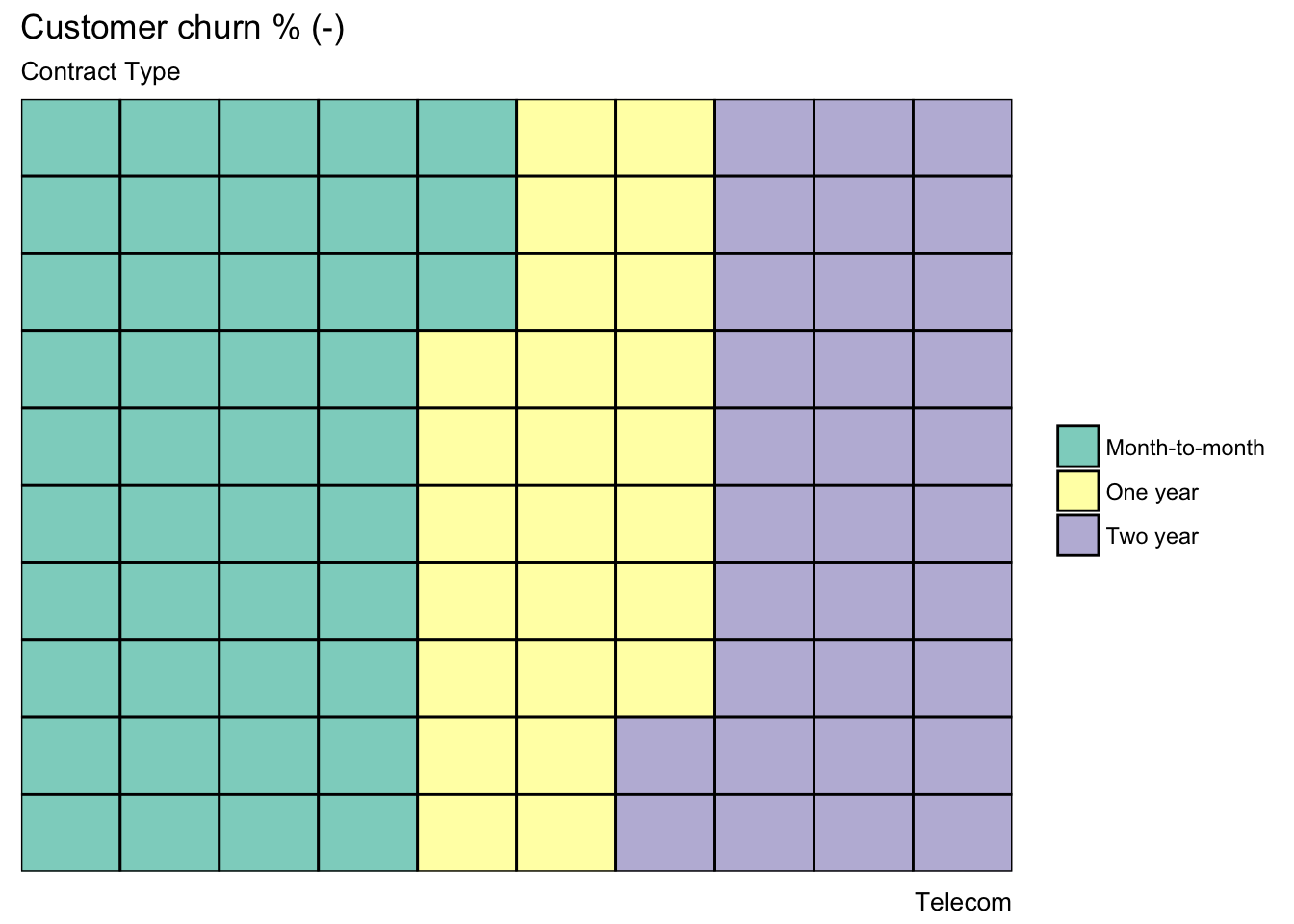
labs(title="Customer churn % (+)", subtitle="Contract Type",
caption="Telecom") +
theme(
plot.title = element_text(size = rel(1.2)),
axis.text = element_blank(),
axis.title = element_blank(),
axis.ticks = element_blank(),
legend.title = element_blank(),
legend.position = "right")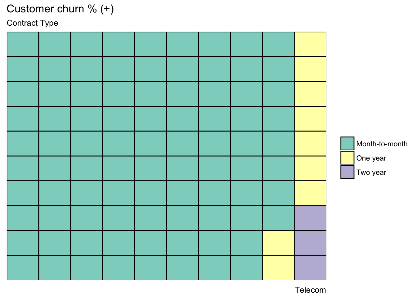
Exploring
plot.barplot(x = churn,
             xname = "Churn",
             fillname = "Contract")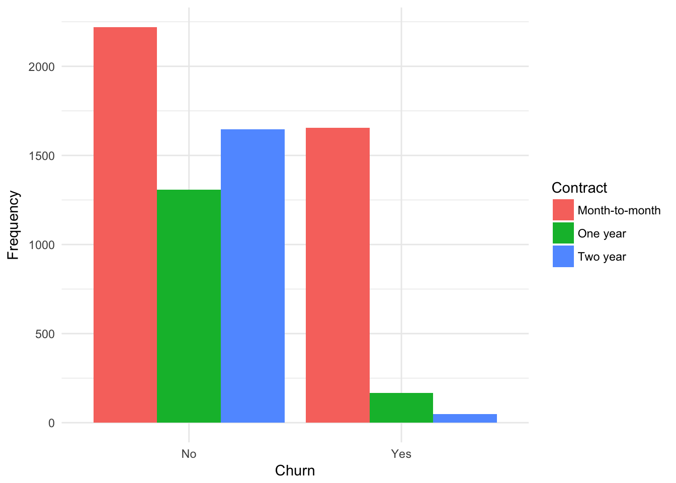
##
##       Month-to-month One year Two year
##   No            2220     1307     1647
##   Yes           1655      166       48
plot.barplot(churn,
xname = "Churn" ,
fillname = "Dependents")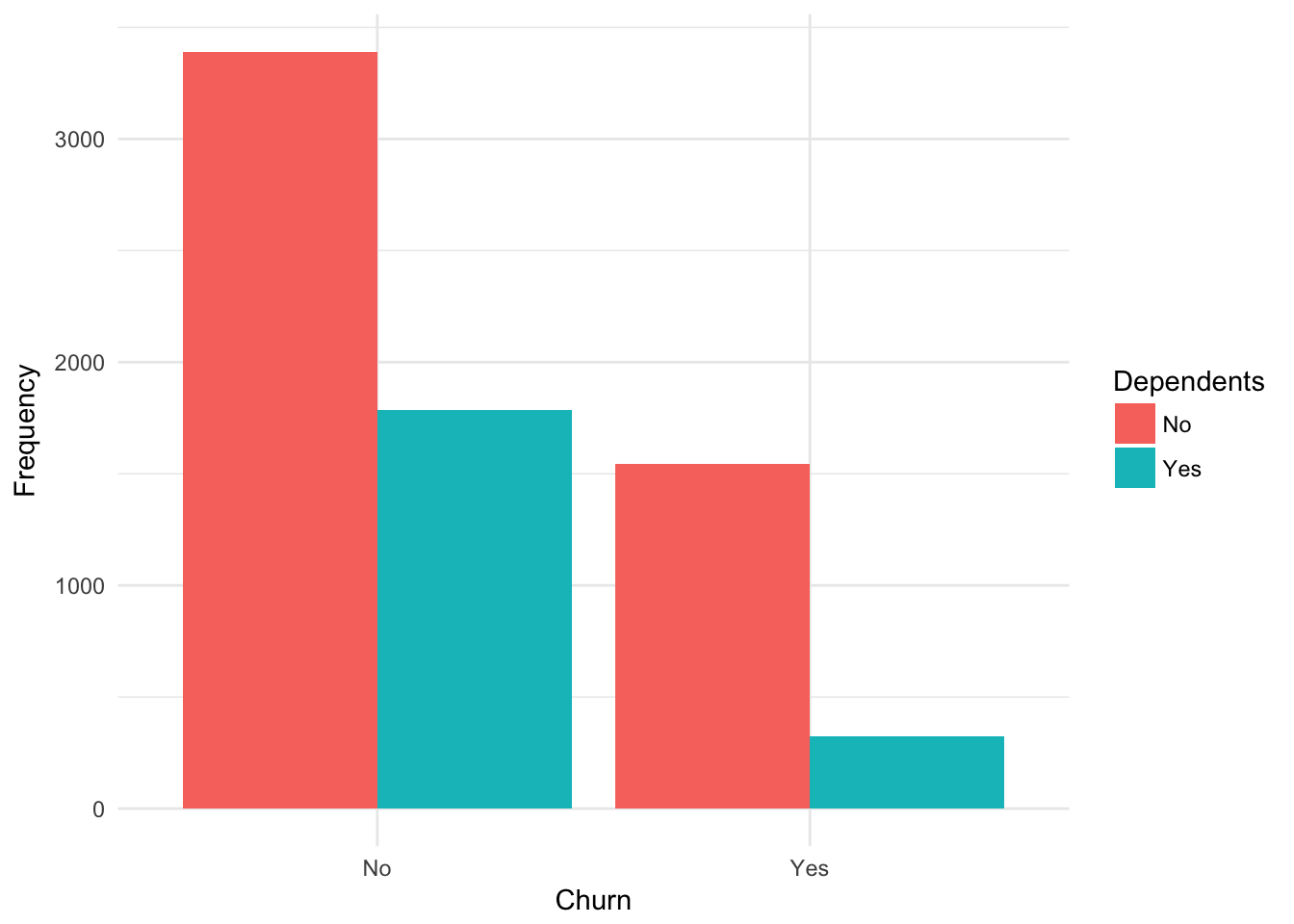
##
##         No  Yes
##   No  3390 1784
##   Yes 1543  326
plot.barplot(churn,
xname = "Churn",
fillname = "StreamingMovies")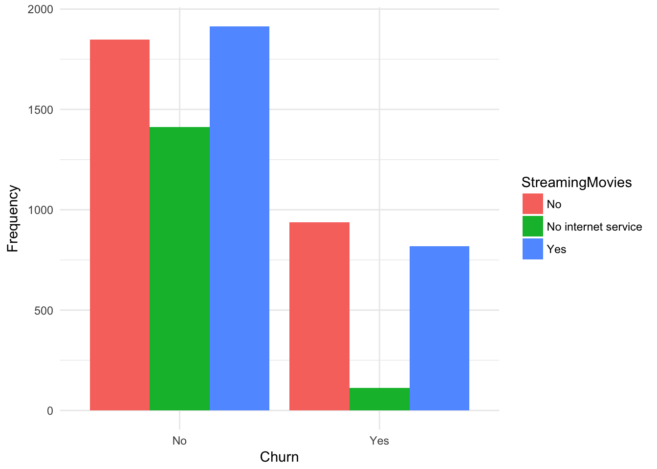
##
##         No No internet service  Yes
##   No  1847                1413 1914
##   Yes  938                 113  818
plot.barplot(churn,
xname = "Churn",
fillname = "PaymentMethod") 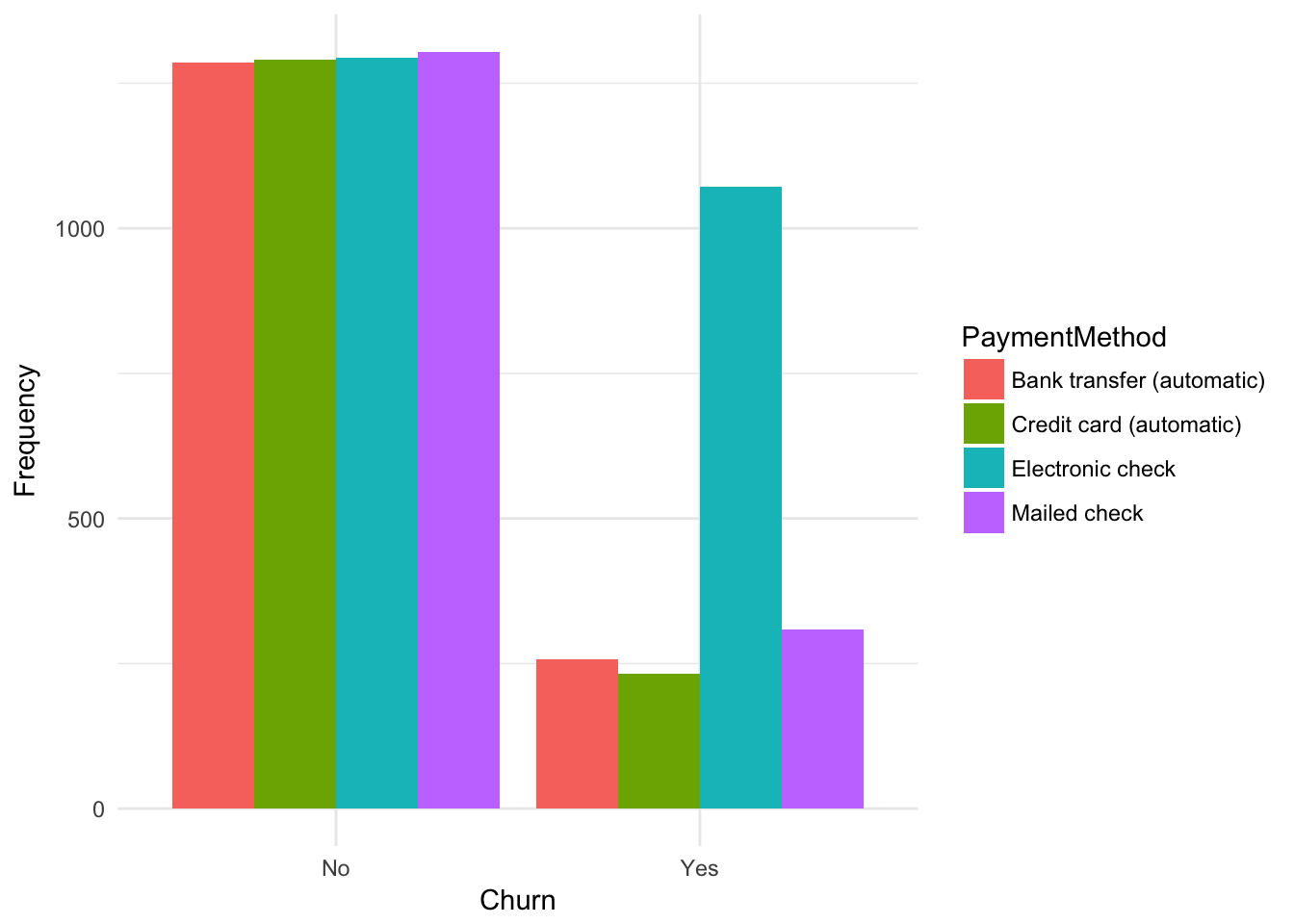
##
##       Bank transfer (automatic) Credit card (automatic) Electronic check
##   No                       1286                    1290             1294
##   Yes                       258                     232             1071
##
##       Mailed check
##   No          1304
##   Yes          308
ggplot(churn, aes(x = Churn, y = tenure, fill= Contract)) +
geom_boxplot() + theme_minimal()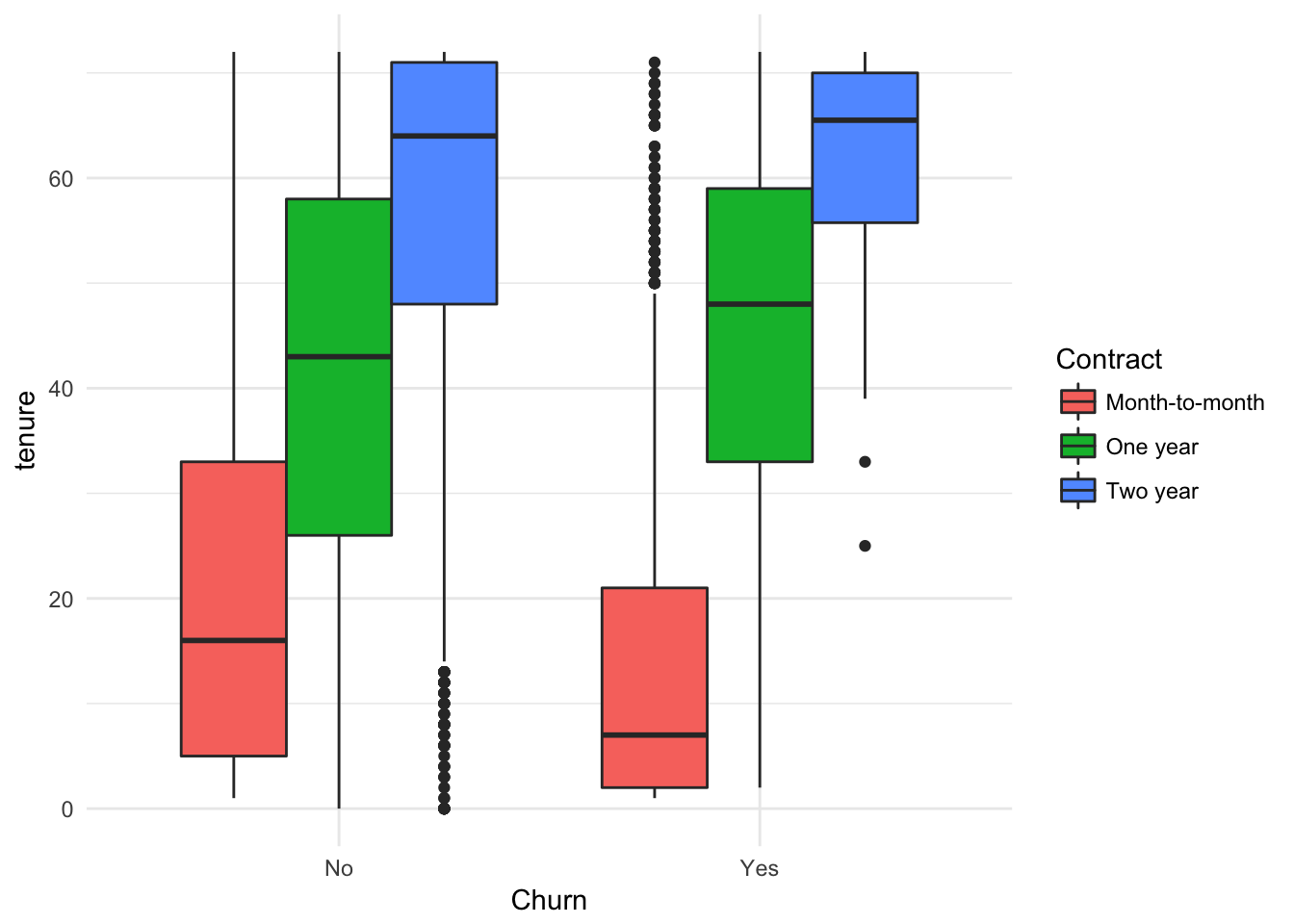
ggplot(churn, aes(x = Churn, y = tenure)) +
  geom_boxplot() + theme_minimal()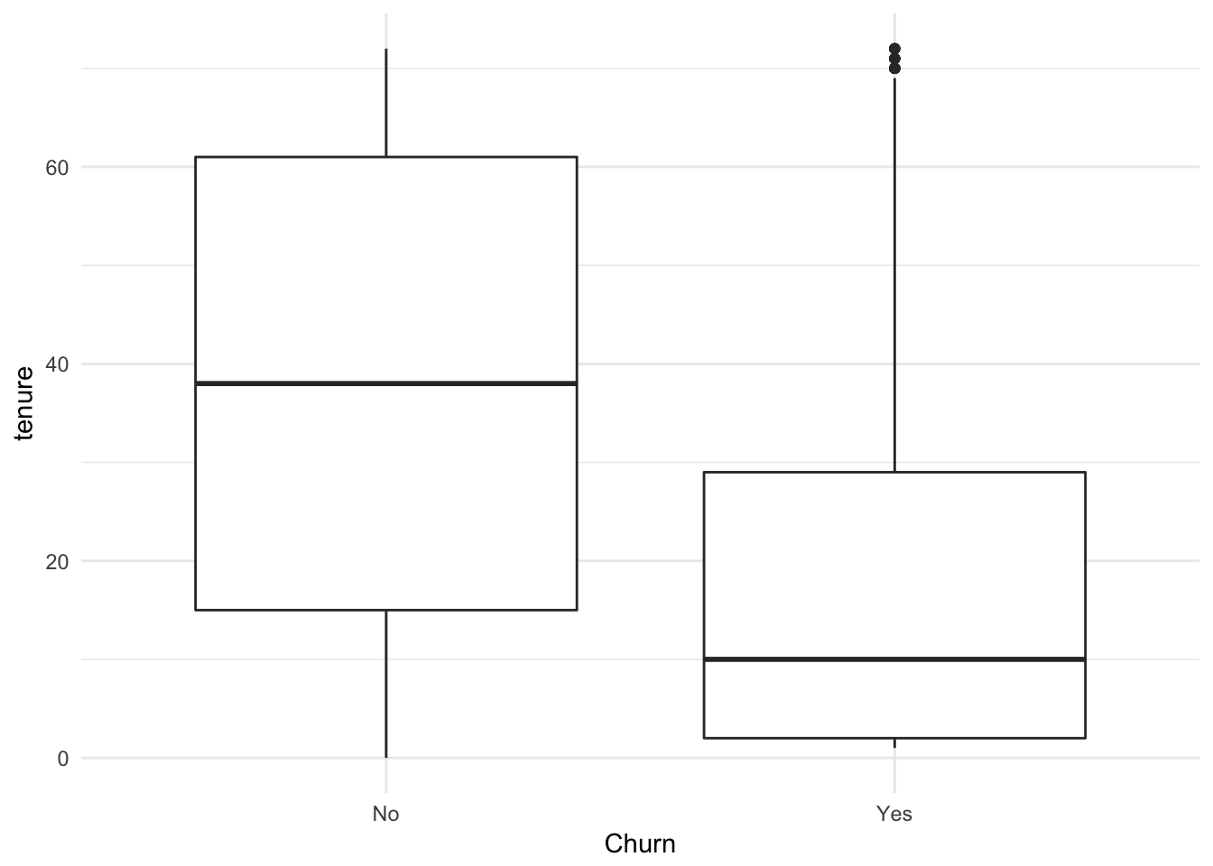
ggplot(churn, aes(x = Churn, y = tenure, fill= TechSupport)) +
  geom_boxplot() + facet_wrap(~SeniorCitizen)+ theme_minimal()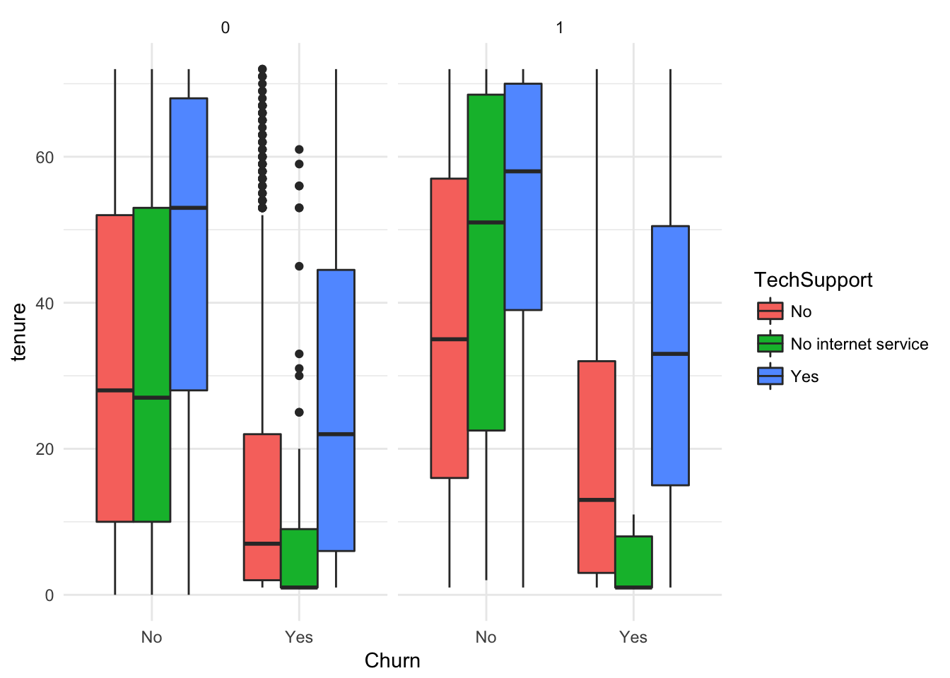
ggplot(churn, aes(x = Churn, y = MonthlyCharges, fill= Contract)) +
  geom_boxplot() + theme_minimal()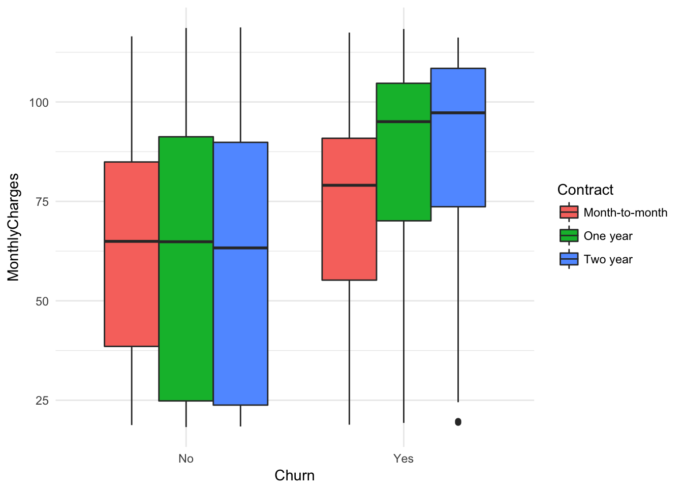
ggplot(churn, aes(x = tenure, y = TotalCharges, color = Contract)) + geom_point( ) + geom_smooth()+ theme_minimal()## `geom_smooth()` using method = 'gam'## Warning: Removed 11 rows containing non-finite values (stat_smooth).## Warning: Removed 11 rows containing missing values (geom_point).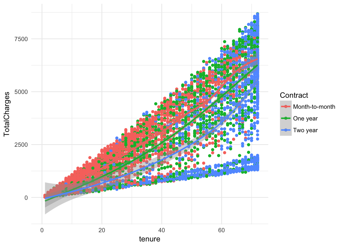
ggplot(churn, aes(x = MonthlyCharges, y = TotalCharges, color = Contract)) + geom_point( ) + geom_smooth()+ theme_minimal()## `geom_smooth()` using method = 'gam'## Warning: Removed 11 rows containing non-finite values (stat_smooth).
## Warning: Removed 11 rows containing missing values (geom_point).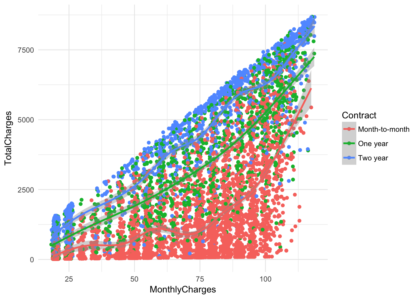
ggplot(churn, aes(x = tenure, y = MonthlyCharges, color = Churn)) +
  geom_point( )+ geom_smooth()+ facet_wrap(~factor(InternetService))+ theme_minimal()
## `geom_smooth()` using method = 'gam'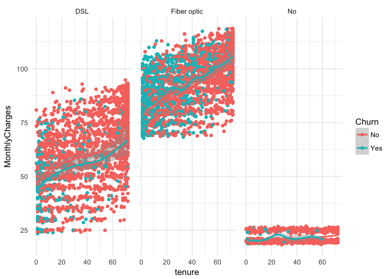
ggplot(churn, aes(x = Churn, y = tenure, fill = InternetService)) +
  geom_boxplot() + facet_wrap(~TechSupport, nrow = 1)+ theme_minimal()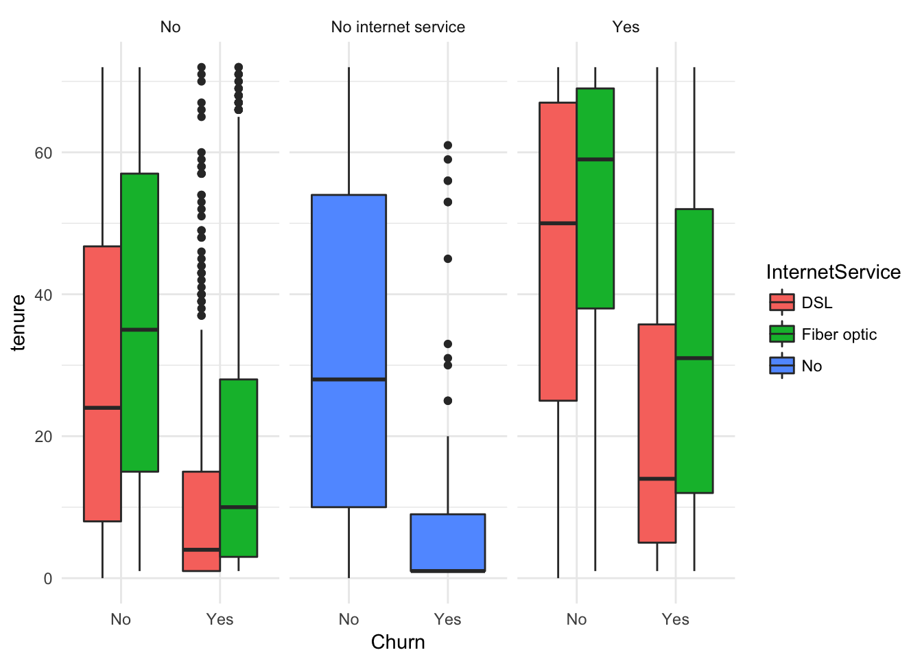
ggplot(churn, aes(x = MonthlyCharges, fill = Churn)) +
  geom_histogram() + theme_minimal()#Monthly Charges by Churn
## `stat_bin()` using `bins = 30`. Pick better value with `binwidth`.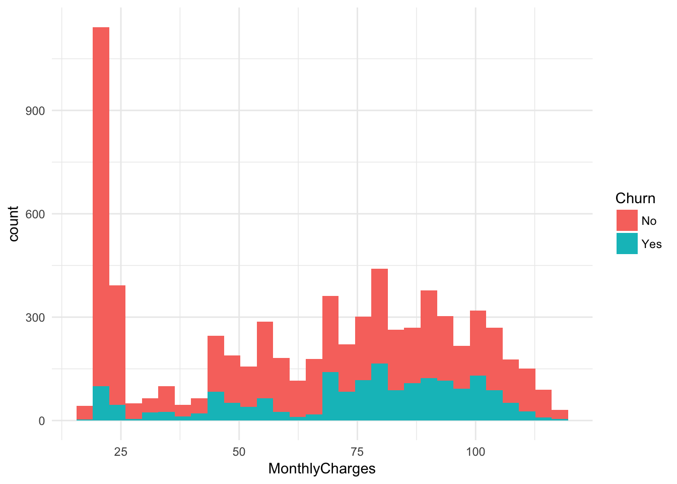
ggplot(churn, aes(x = MonthlyCharges, fill = TechSupport)) +
  geom_histogram() + theme_minimal()
## `stat_bin()` using `bins = 30`. Pick better value with `binwidth`.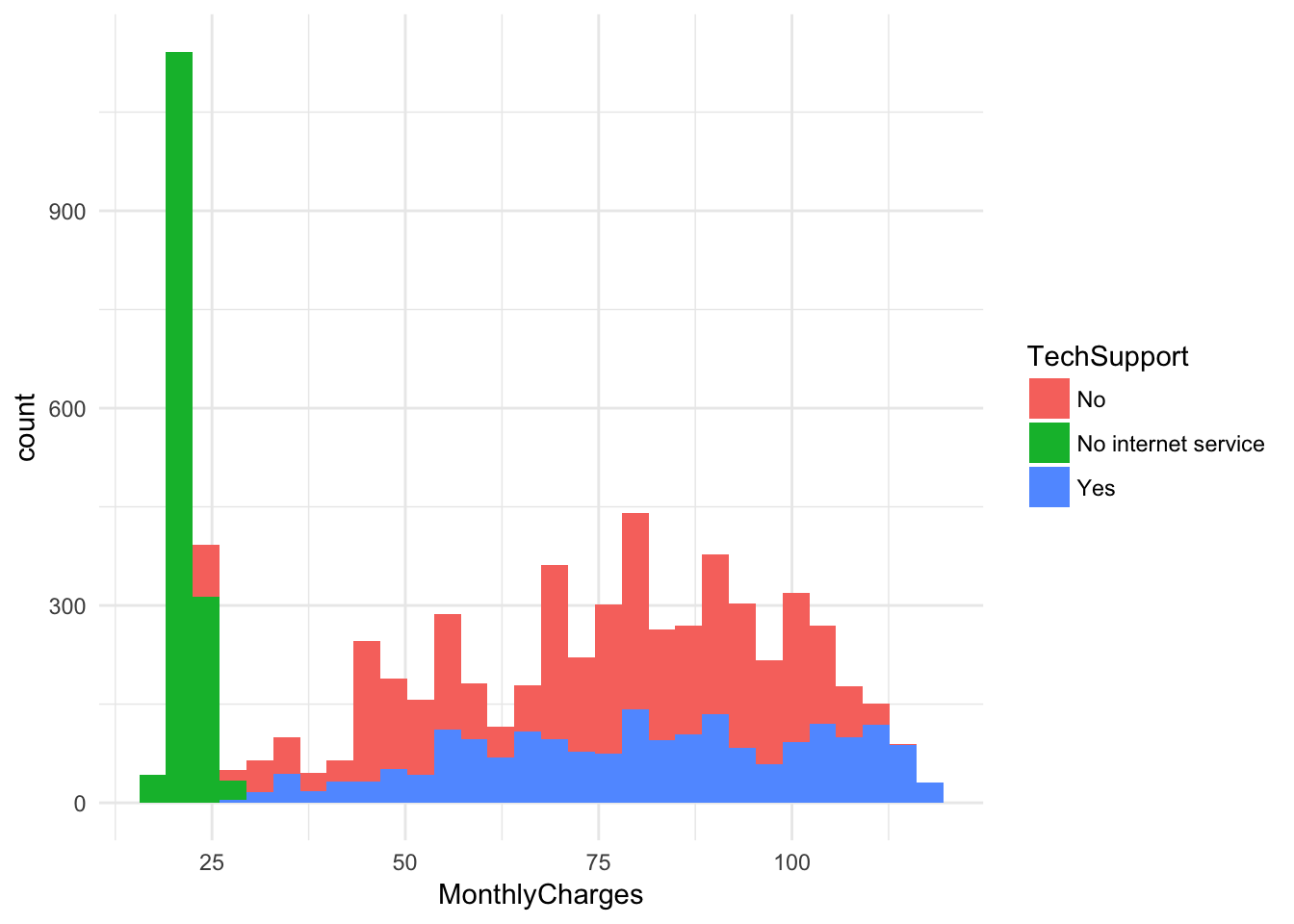
ggplot(churn, aes(x = MonthlyCharges, fill = InternetService)) +
  geom_histogram() + theme_minimal()
## `stat_bin()` using `bins = 30`. Pick better value with `binwidth`.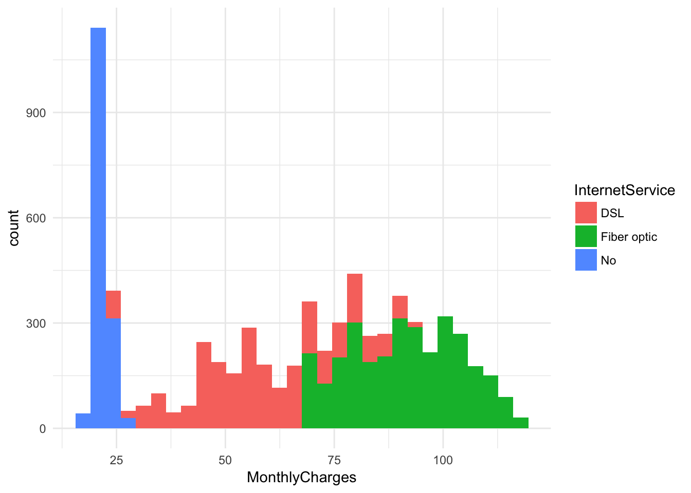
ggplot(churn, aes(x = TotalCharges, fill = Contract)) +
  geom_histogram() + facet_wrap(~InternetService) + theme_minimal()
## `stat_bin()` using `bins = 30`. Pick better value with `binwidth`.## Warning: Removed 11 rows containing non-finite values (stat_bin).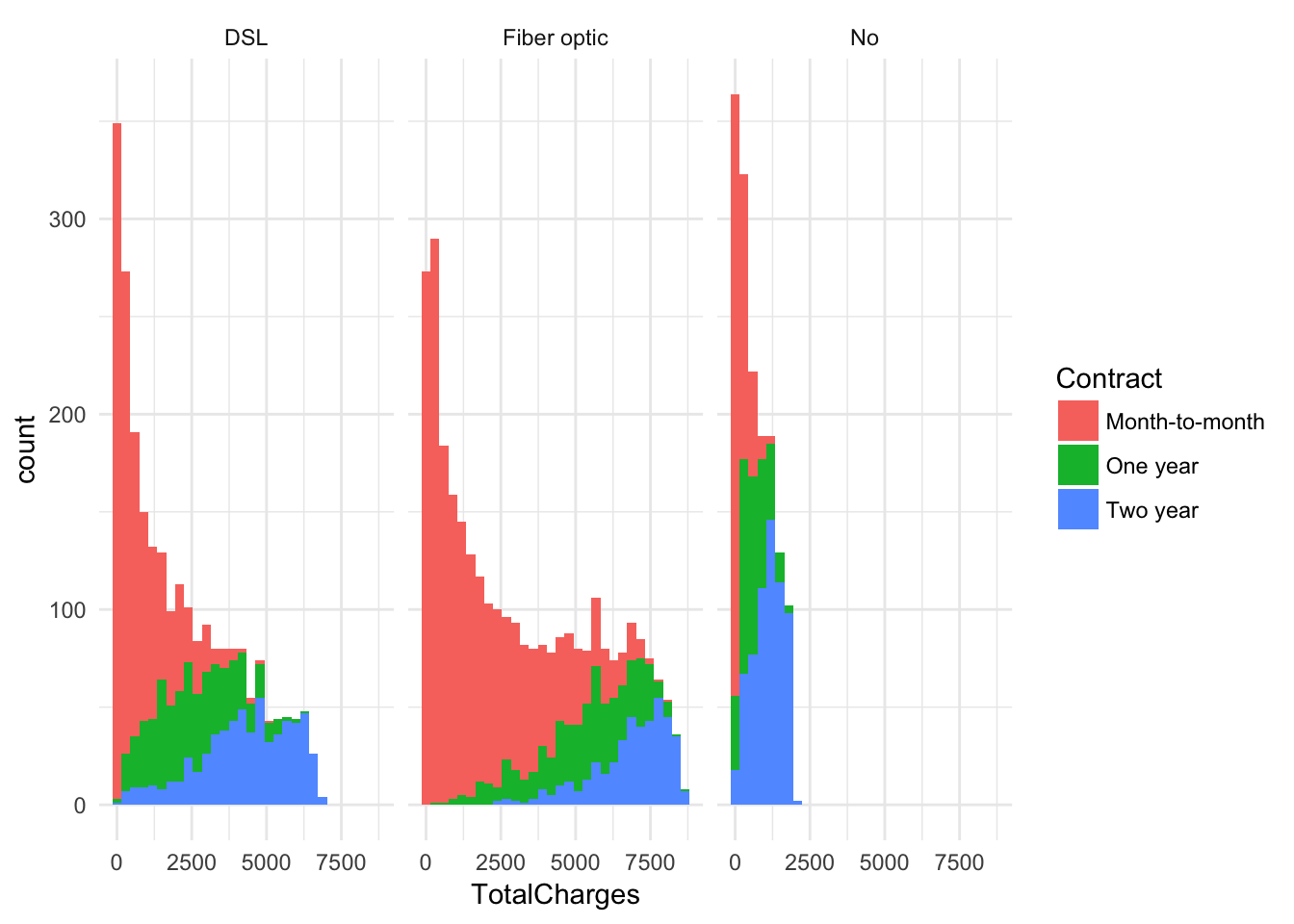
 ggplot(churn, aes(x = tenure, y = MonthlyCharges, color = InternetService)) +
  geom_point( )+ geom_smooth()+ theme_minimal()
## `geom_smooth()` using method = 'gam'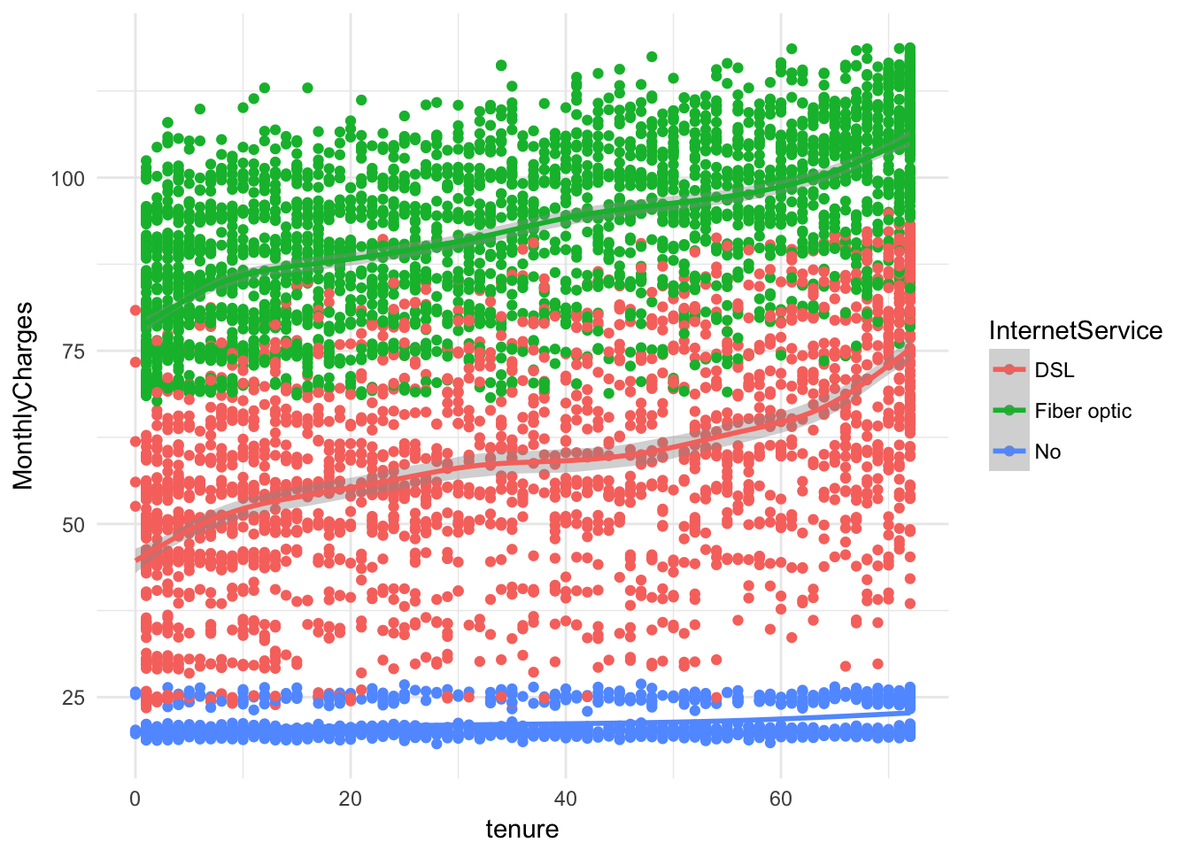
Model Building
For this mini-project, we will use logistic regression, decision trees, and k-nearest neighbors.
set.seed(100)
indx <- sample(1:nrow(churn), .8*nrow(churn), replace = F)
Logistic Regression
Since I am only using logistic regression to explore relationships, and I’m not necessarily too concerned with the accuracy of this particular model, I will hold off on splitting the data 80-20 until the subsequent models.
churn$Churn <- factor(churn$Churn)
churn$SeniorCitizen <- factor(churn$SeniorCitizen )
fit <- glm(Churn ~ SeniorCitizen + MonthlyCharges + tenure + Contract +
             PaymentMethod +TechSupport, data = churn, family = "binomial")
summary(fit)
##
## Call:
## glm(formula = Churn ~ SeniorCitizen + MonthlyCharges + tenure +
## Contract + PaymentMethod + TechSupport, family = "binomial",
## data = churn)
##
## Deviance Residuals:
## Min 1Q Median 3Q Max
## -1.8322 -0.6735 -0.3045 0.7601 3.1709
##
## Coefficients:
## Estimate Std. Error z value Pr(>|z|)
## (Intercept) -1.330859 0.149909 -8.878 < 2e-16
## SeniorCitizen1 0.349465 0.081552 4.285 1.83e-05
## MonthlyCharges 0.022466 0.001796 12.508 < 2e-16
## tenure -0.034080 0.002107 -16.174 < 2e-16
## ContractOne year -0.812642 0.103350 -7.863 3.75e-15
## ContractTwo year -1.560966 0.171277 -9.114 < 2e-16
## PaymentMethodCredit card (automatic) -0.060629 0.112223 -0.540 0.589023
## PaymentMethodElectronic check 0.424624 0.092594 4.586 4.52e-06
## PaymentMethodMailed check -0.068929 0.111202 -0.620 0.535353
## TechSupportNo internet service -0.484025 0.142733 -3.391 0.000696
## TechSupportYes -0.536799 0.082908 -6.475 9.51e-11
##
## (Intercept) ***
## SeniorCitizen1 ***
## MonthlyCharges ***
## tenure ***
## ContractOne year ***
## ContractTwo year ***
## PaymentMethodCredit card (automatic)
## PaymentMethodElectronic check ***
## PaymentMethodMailed check
## TechSupportNo internet service ***
## TechSupportYes ***
## ---
## Signif. codes: 0 '***' 0.001 '**' 0.01 '*' 0.05 '.' 0.1 ' ' 1
##
## (Dispersion parameter for binomial family taken to be 1)
##
## Null deviance: 8150.1 on 7042 degrees of freedom
## Residual deviance: 6000.7 on 7032 degrees of freedom
## AIC: 6022.7
##
## Number of Fisher Scoring iterations: 6exp(coef(fit))## (Intercept) SeniorCitizen1
## 0.2642503 1.4183090
## MonthlyCharges tenure
## 1.0227206 0.9664939
## ContractOne year ContractTwo year
## 0.4436841 0.2099333
## PaymentMethodCredit card (automatic) PaymentMethodElectronic check
## 0.9411728 1.5290152
## PaymentMethodMailed check TechSupportNo internet service
## 0.9333929 0.6162979
## TechSupportYes
## 0.5846168exp(cbind(OR = coef(fit), confint(fit)))## Waiting for profiling to be done...## OR 2.5 % 97.5 %
## (Intercept) 0.2642503 0.1966656 0.3539899
## SeniorCitizen1 1.4183090 1.2087080 1.6641164
## MonthlyCharges 1.0227206 1.0191468 1.0263494
## tenure 0.9664939 0.9624845 0.9704687
## ContractOne year 0.4436841 0.3615988 0.5423228
## ContractTwo year 0.2099333 0.1485725 0.2911130
## PaymentMethodCredit card (automatic) 0.9411728 0.7551599 1.1726155
## PaymentMethodElectronic check 1.5290152 1.2760141 1.8345824
## PaymentMethodMailed check 0.9333929 0.7507904 1.1611240
## TechSupportNo internet service 0.6162979 0.4650220 0.8139424
## TechSupportYes 0.5846168 0.4965972 0.6873646Some intersting things to point out: based on the data, those who pay with elecronic check have a 50% higher odds of churning over the baseline. Moreover, a one unit increase in montly charges cost corresponds with a 2% greater odds of churning.
tree = rpart::rpart(Churn ~ SeniorCitizen + MonthlyCharges + tenure + Contract +
               PaymentMethod +TechSupport + Dependents , data = churn)
rpart.plot::rpart.plot(tree)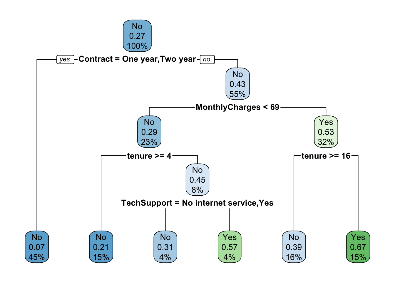
train <- churn[indx,c("MonthlyCharges", "tenure", "TotalCharges", "Churn")]
test <- churn[-indx,c("MonthlyCharges", "tenure", "TotalCharges", "Churn")]

train <- na.omit(train)
test <- na.omit(test)
kn <- class::knn(train[,-4], test[,-4],train[,4] , k = 22, l = 4, prob = F, use.all = TRUE)
length(kn)
## [1] 1408dim(test)## [1] 1408 4df <- table(Prob = kn, Obs = test[,"Churn"]) %>% data.frame()
ggplot(df, aes(x = Prob, y = Freq, fill = Obs)) +
geom_bar(stat = 'identity', position = "dodge") + theme_light()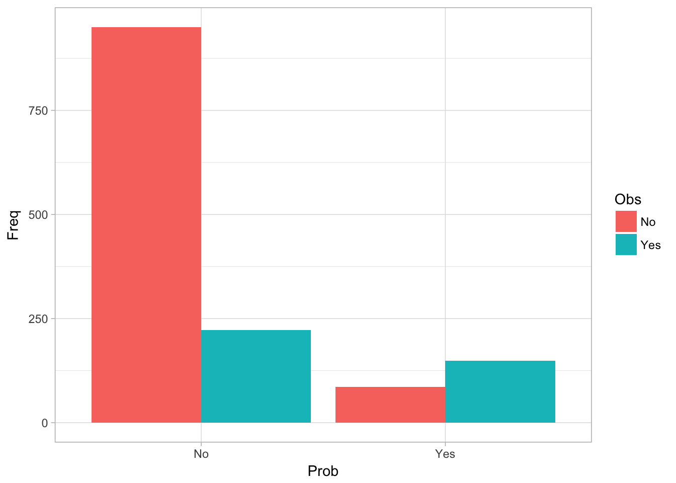
table(Prob = kn, Obs = test[,"Churn"])## Obs
## Prob No Yes
## No 950 223
## Yes 86 149table(Prob = kn, Obs = test[,"Churn"]) %>% prop.table()## Obs
## Prob No Yes
## No 0.67471591 0.15838068
## Yes 0.06107955 0.10582386This final model was able to achieve about 80% accuracy. KNN is very competitve with logistic regression and decision trees out of the box model.