Mixed Effects & Air Fares
By Jamel Thomas
In the United States, various factors affect the airfare prices that consumers see. An issue is that a single linear model may not fit the data, as prices can vary drastically across different routes. We will obtain Quarterly US Air Fare and Volume data and utilize a mixed effects model to predict air fare prices. The original dataset contains 108,602 observations and 14 attributes and there are no missing values. For the sake of simplicity, in this paper, we only consider a random sample of 50 routes as the original dataset contains 4177 routes.
library(ggplot2)
library(ggmap)
library(nlme)
library(lattice)
library(MASS)
library(corrplot)
## corrplot 0.84 loadeddist <- read.table(file = "http://stat.ufl.edu/~winner/data/distang26.dat",
col.names = c("Airport1", "Airport2", "Population1", "Population2",
"Distance", "Angle", "Latitude.City1", "Latitude.City2",
"Longitude.City1", "Longitude.City2"))
rout <- read.table("http://www.stat.ufl.edu/~winner/data/longair.dat")
colnames(rout) <- c("Route", "Quarter", "Avg.Fare", "Avg.Pass")
data.both <- cbind(rout, dist)
head(rout, 10)## Route Quarter Avg.Fare Avg.Pass
## 1 1 1 198.96 72.50
## 2 1 2 205.00 91.30
## 3 1 3 230.46 76.77
## 4 1 4 216.53 121.31
## 5 1 5 221.16 91.63
## 6 1 6 235.97 95.00
## 7 1 7 265.75 78.11
## 8 1 8 234.43 99.01
## 9 1 9 204.96 97.17
## 10 1 10 203.77 108.47Moreover, for every route, there are 26 quarters for which the average fare price is taken. Therefore, we simplify the problem dramatically with the exclusion of most of the routes. Our objective is to build a linear mixed effects model to predict the average fare price for each route.
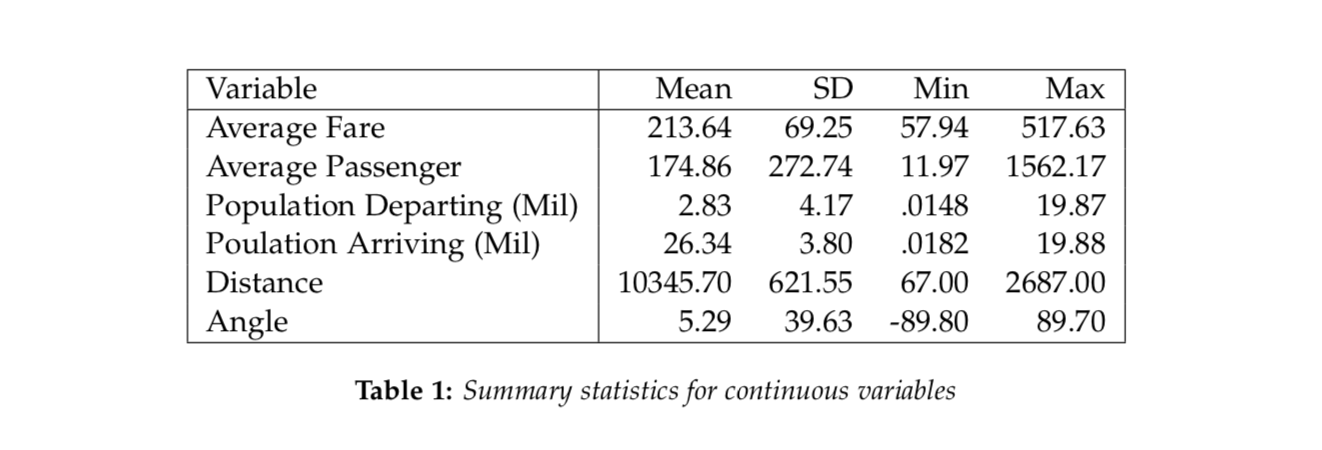
It’s unknown how the data was collected, but I assumed that the data is obtained from one airline company. The response variable is the Average Fare. The covariates include the route number, the quarter, average weekly passengers, departing airport, arrival airport, the population of the departing city, the population of the arrival city, the distance traveled, the angle of the route, and the longitude and latitude of both departing and arriving airports. Table 1 shows the summary statistics for the subsetted dataset.
We considered a linear mixed effects model with a random intercept route term for the randomly selected routes. This is fitted on log-transformation of average fares and we consider all covariates without interaction. In the appendix, we justify using a log-transformation rather than a box-cox transformation of the data. The essence is that there is not much gained from the box-cox transformation over the logarithm. Moreover, the Normal Q-Q plot for the log-transformed response appears to have about the same skewness as the Box-Cox.
attach(rout)
hist(rout$Avg.Fare) 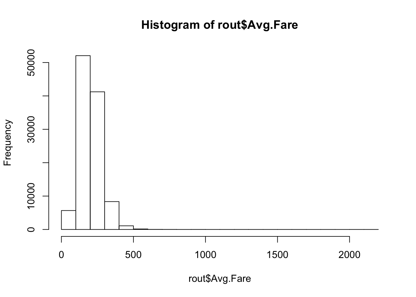
hist(log(rout$Avg.Fare)) 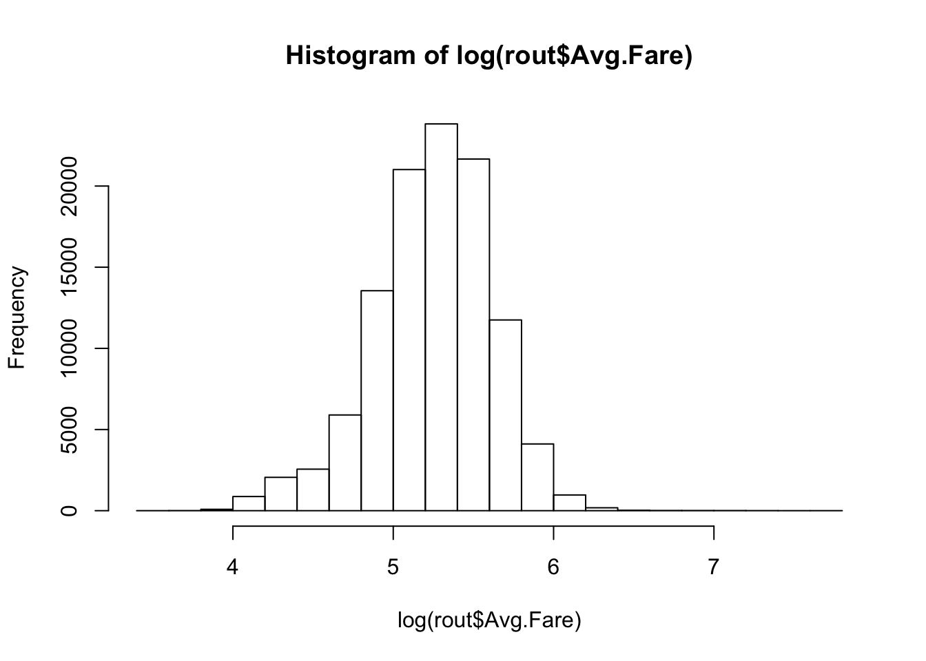
box <- MASS::boxcox(rout$Avg.Fare~ rout$Quarter + rout$Avg.Pass, data = rout) #Boxcox 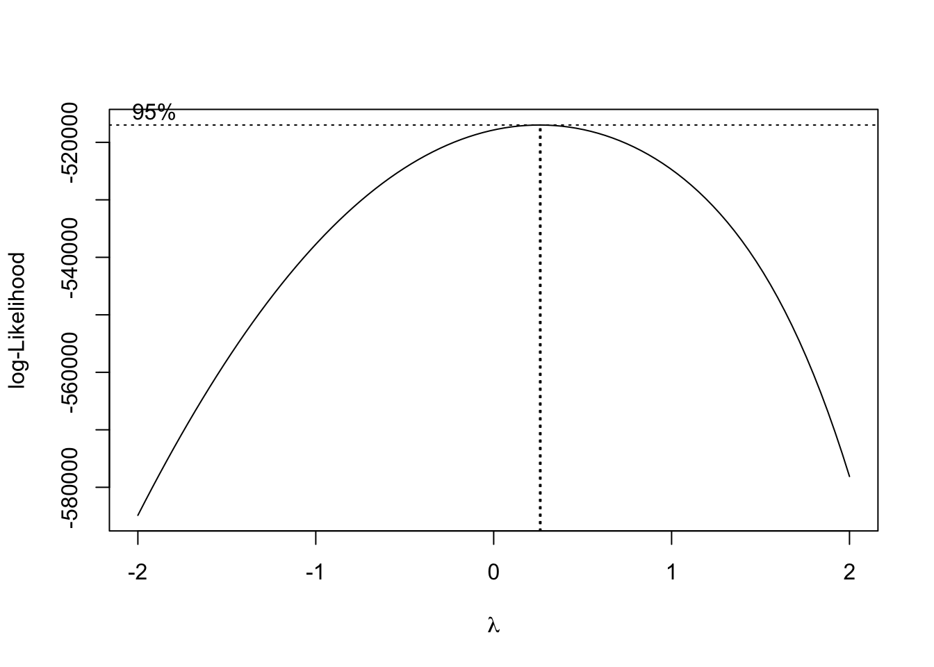
print(max.bc <- box$x[box$y==max(box$y)])## [1] 0.2626263newFare <- (rout$Avg.Fare^max.bc - 1)/(max.bc)
hist(newFare)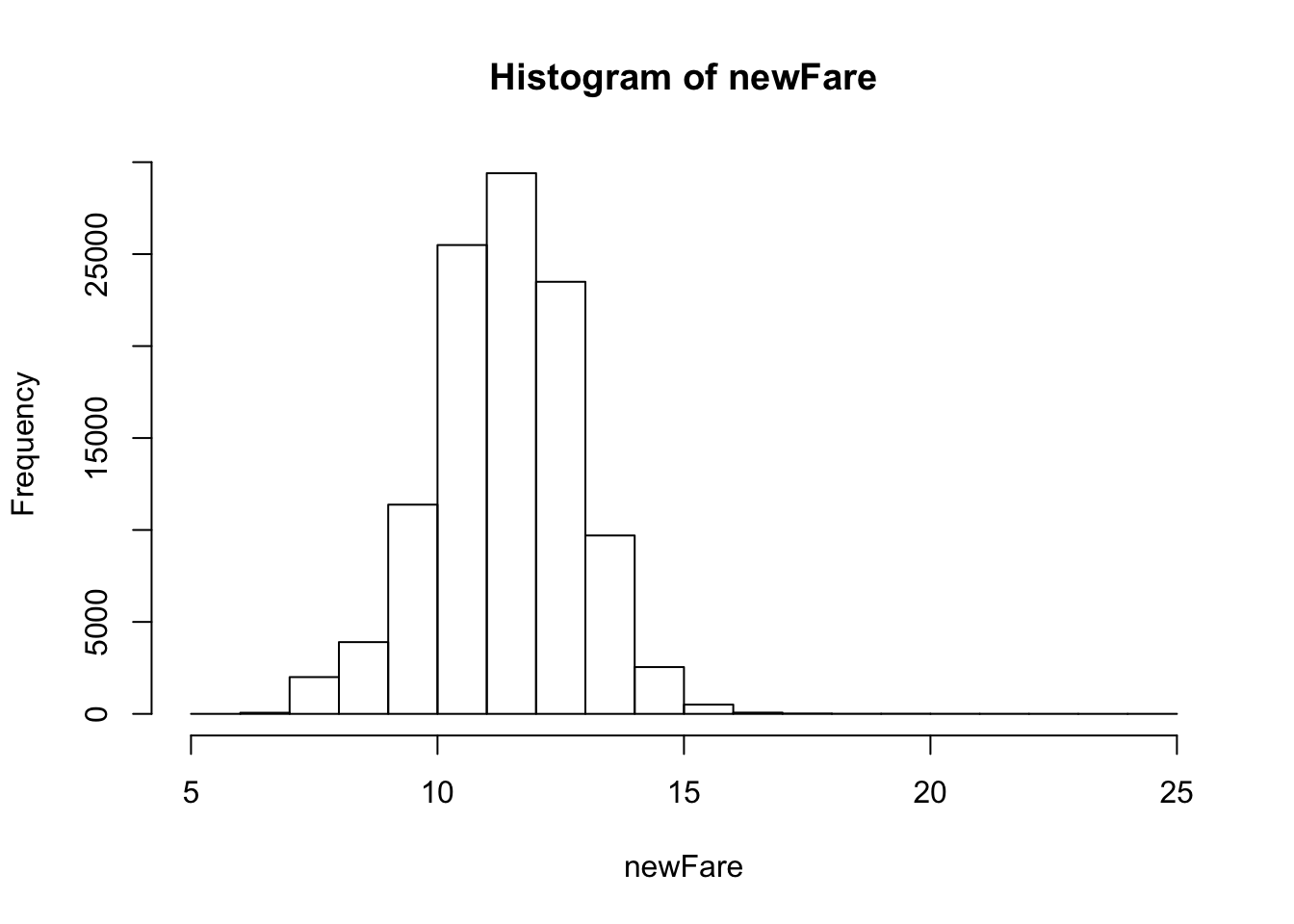
qqnorm(newFare)
qqline(newFare) #The log-transform is more simple, we will use log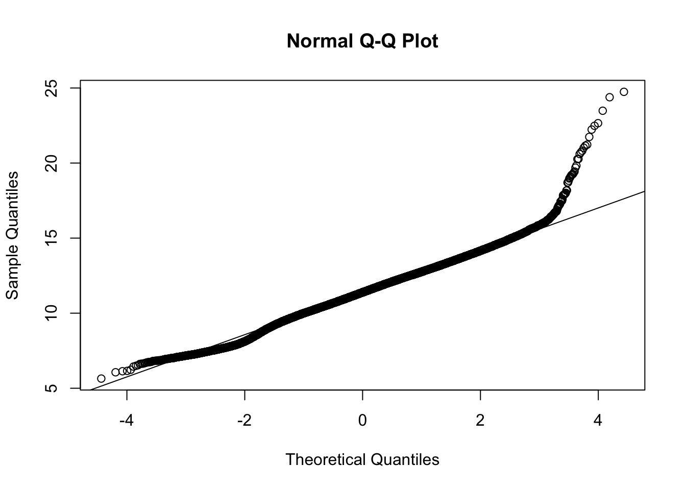 We attempted to aggregate the data by combining all common quarters together. This means that the data was divided into 4 quarters in terms of the business quarters for each year. The leftover 2 quarters were included in this dataset. When we attempted to fit a model to this data it did not yield better results than the original time-scale. We did the same thing with a yearly time-scale but were met with the same results.
log.lme <- lme(log(Avg.Fare) ~ Quarter + I(Quarter^2)+ Avg.Pass ,
     data = sub2, random = ~1|Route) #The model
plot(log.lme)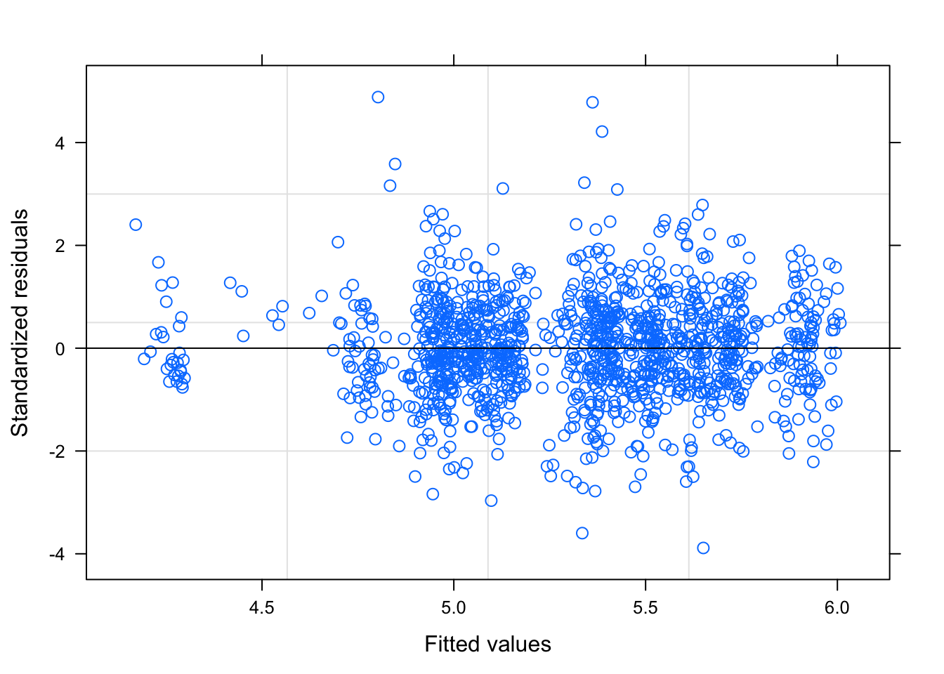
par(mfrow=c(1,1))
qqnorm(resid(log.lme)); qqline(resid(log.lme), col = "red")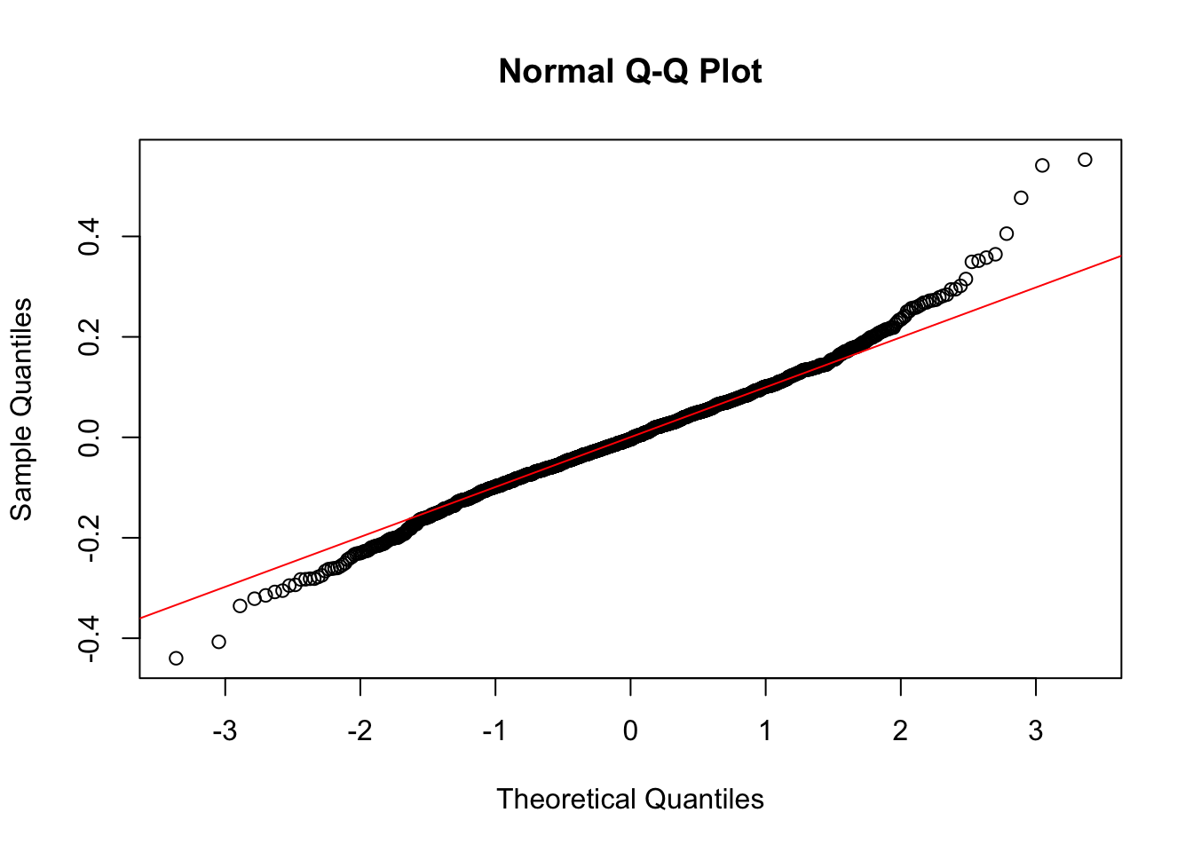
summary(log.lme)## Linear mixed-effects model fit by REML
## Data: sub2
## AIC BIC logLik
## -1643.077 -1612.074 827.5383
##
## Random effects:
## Formula: ~1 | Route
## (Intercept) Residual
## StdDev: 0.3364873 0.1131828
##
## Fixed effects: log(Avg.Fare) ~ Quarter + I(Quarter^2) + Avg.Pass
## Value Std.Error DF t-value p-value
## (Intercept) 5.334042 0.04930513 1247 108.18433 0
## Quarter 0.013740 0.00173972 1247 7.89764 0
## I(Quarter^2) -0.000509 0.00006261 1247 -8.12464 0
## Avg.Pass -0.000941 0.00008667 1247 -10.85284 0
## Correlation:
## (Intr) Quartr I(Q^2)
## Quarter -0.180
## I(Quarter^2) 0.152 -0.970
## Avg.Pass -0.161 -0.016 0.049
##
## Standardized Within-Group Residuals:
## Min Q1 Med Q3 Max
## -3.88627078 -0.58795127 -0.03295835 0.59642315 4.88443734
##
## Number of Observations: 1300
## Number of Groups: 50Building this model, we considered a random slope for routes. When the analysis was run the random slope was found to be statistically significant but it was not practically significant. Therefore, the random slope was dropped from the model. We also considered a quadratic term for average passengers. This was also found to be statistically significant but not practically significant. Therefore, it was excluded from the model. The final model contains the covariates quarter, log-average passenger, quarter squared and a random intercept effect for route.
In conclusion, we obtain a model with linear mixed effects on Route. We began with exploratory analysis of the response variable and found the best, simple, model has a quadratic term of Quarter and log-Average Passengers. For every one unit increase in Quarter, we obtain about a 2% increase in Average Fare, assuming all other covariates are fixed. Moreover, For every one unit increase in Average Passengers per week, we obtain about a 25.9% decrease in Average Fare, assuming all other covariates are fixed. This may be because an increase in passengers allows the airline to lower fare prices. The standard deviation is nearly 0.4 on the log-scale, with residuals around 0.12. None of the confidence intervals contain zero, which verifies their significance in the model. The model may not be the best fit, as it obtains an MSE for observed vs predicted of 792.5. There may be a better model for this dataset, however, the simple model is the most convenient. To improve efficiency more covariates may be needed. Finally, since the model was built on a subset based on routes and it is not perfect, the model does not generalize well to the entire dataset.
Notes
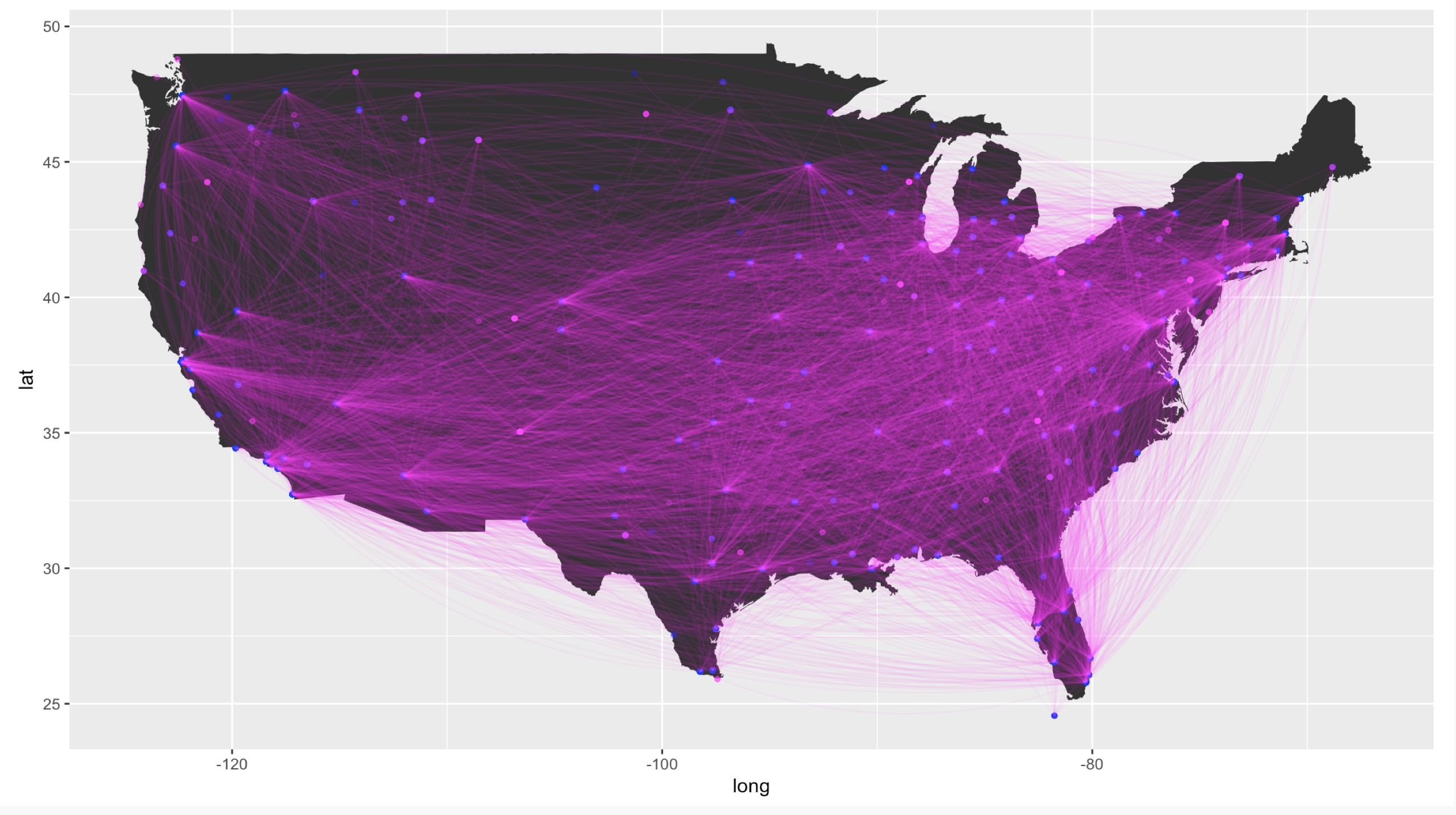
Just as a side point, here is the code used to build the map in the beginning of this blog post.
states <- map_data("usa")
p <- ggplot() + geom_polygon(data = states, aes(x=long, y = lat, group = group)) +
  coord_fixed(1.3) +
  geom_point(data = dist, aes(x = dist$Longitude.City1, y = dist$Latitude.City1),
             color = rgb(1,0,1,1/4), size = 1) +
  geom_point(data = dist, aes(x = dist$Longitude.City2, y = dist$Latitude.City2),
             color = rgb(0,0,1,1/4), size = 1)
p + geom_curve(aes(x = dist$Longitude.City1, y = dist$Latitude.City1,
                   xend = dist$Longitude.City2, yend = dist$Latitude.City2),
               data = dist, curvature = -.2, colour = rgb(1,0,1, .05))